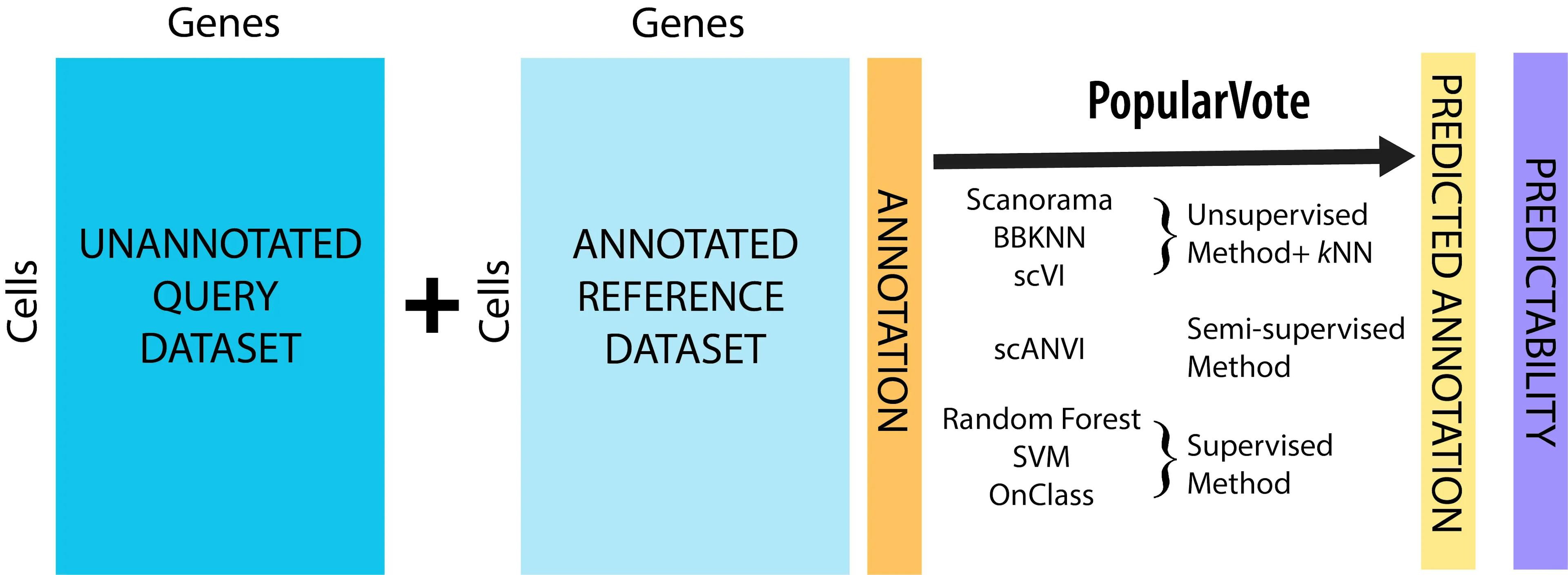
We call our annotation pipeline popularVote (popV for short). The idea behind popV is not to tie the annotation process to one particular annotation algorithm. Instead, popV applies a series of annotation algorithms, each providing a different recipe for transferring labels from Tabula Sapiens to the user-provided data. popV then conducts consensus analysis over these algorithms to estimate the most reproducible annotation of every cell, and to highlight cells that are difficult to label (where the algorithms disagree). These cells are highlighted to the user as requiring a more in-depth inspection.

By using this online collab notebook users can bring their own scRNAseq datasets with no prior labeling and generate cell type predictions. The dataset should contain a raw count matrix (unnormalized integer counts) or processed to remove ambient RNA contamination if desired (unnormalized rounded counts). For best performance, we recommend that, if desired, users select the physiologically closest organ available as their reference.

Annotate user dataset

Tabula Sapiens dataset is curated according to current best practices in bioinformatics and annotated by a team of biologists with domain-specific knowledge. All the labels in the dataset use the OBO Foundry candidate ontology Cell Ontology (CL) vocabulary.

Launch collab session

What does the annotation pipeline include?

• Our pipeline performs automated cell type annotation using seven different annotation methods. We chose these methods because they have good prediction accuracy in (Abdelaal et al. 2019) and/or good harmonization performances (Luecken et al. 2020). Users can specify a subset of these methods if they find some of them to be less applicable to their dataset.
• Our pipeline also provides a consensus classifier that aggregates the calls made by the different methods. In addition to increasing accuracy, the consensus statistics helps highlighting groups of cells in which the annotation is uncertain and that should be inspected manually.
• Our collection of annotation methods includes: standard classifiers (random forest (RF), support vector machine (SVM)), single cell-specific annotation methods (scANVI (Xu et al. 2021), and onClass (Wang et al. 2020)), and k nearest neighbours (kNN) in a joint space where the query data is integrated with Tabula Sapiens. We implemented three different integration methods (scVI (Lopez et al. 2018), BBKNN (Polański et al. 2020), and Scanorama (Hie et al. 2019)) and treat each as a different classifier. We leverage scArches (Lotfollahi et al. 2021) reference mapping to integrate query datasets in to the pertained scVI and scANVI reference models. We also compute the consensus prediction using the input from all the methods.

Setup

• Open the colab notebook
• Make sure GPU is enabled (Runtime -> Change Runtime Type-> Hardware Accelerator -> GPU)
• If possible, sign up for a Colab PRO account for higher RAM.

Example data set

You can download a subsampled version of the data reported in Lung Cell Atlas (Travaglini et al. 2020) as an example query data within the notebook.

Input data

Format: the input data should be a .h5ad file. It can be loaded in the notebook using the following three options:

• Connecting to google drive
• Downloading from the cloud
• Uploading manually using the folder icon on the left navigation bar, and selecting the upload icon

Preprocessing requirement

• Cell filtering: for best performance, doublets and low quality cells should be removed before inputting the data
• Raw UMI counts: our annotation pipeline contains methods that models raw UMI counts (scVI and scANVI) and handles the normalization for the other methods internally.
• Normalize for gene length for non-UMI, full length sequencing

Output

Finding the output files

Output files are located in the save folder defined by the user at the beginning of Step 3 in the collab notebook.

• If the save folder starts with ‘./’ the output files are found in the folder icon on the left navigation bar (by default).
• If you’d like to save the output files to your google drive folder you can change the save folder to start with '/content/drive/MyDrive/'.

You can find two .h5ad files:

• Annotated_query.h5ad contains the annotated query dataset
• annotated_query_plus_ref.h5ad contains the annotated query dataset in a harmonized latent space with the reference dataset

You can visualize the latent space of the annotated h5ad files in CZ CELLxGENE.

Format columns of output .obs dataframe

We preserve the metadata column from both query and reference data.

Each method prediction is saved (knn_on_bbknn_pred, knn_on_scvi_offline_pred, scanvi_offline_pred, svm_pred, rf_pred, onclass_pred, knn_on_scanorama_pred).

The majority vote result that is our recommended prediction to use is in the column ‘consensus_prediction’ and the concensus percentage is in the column ‘consensus_percentage’.

Figures generated by the notebook

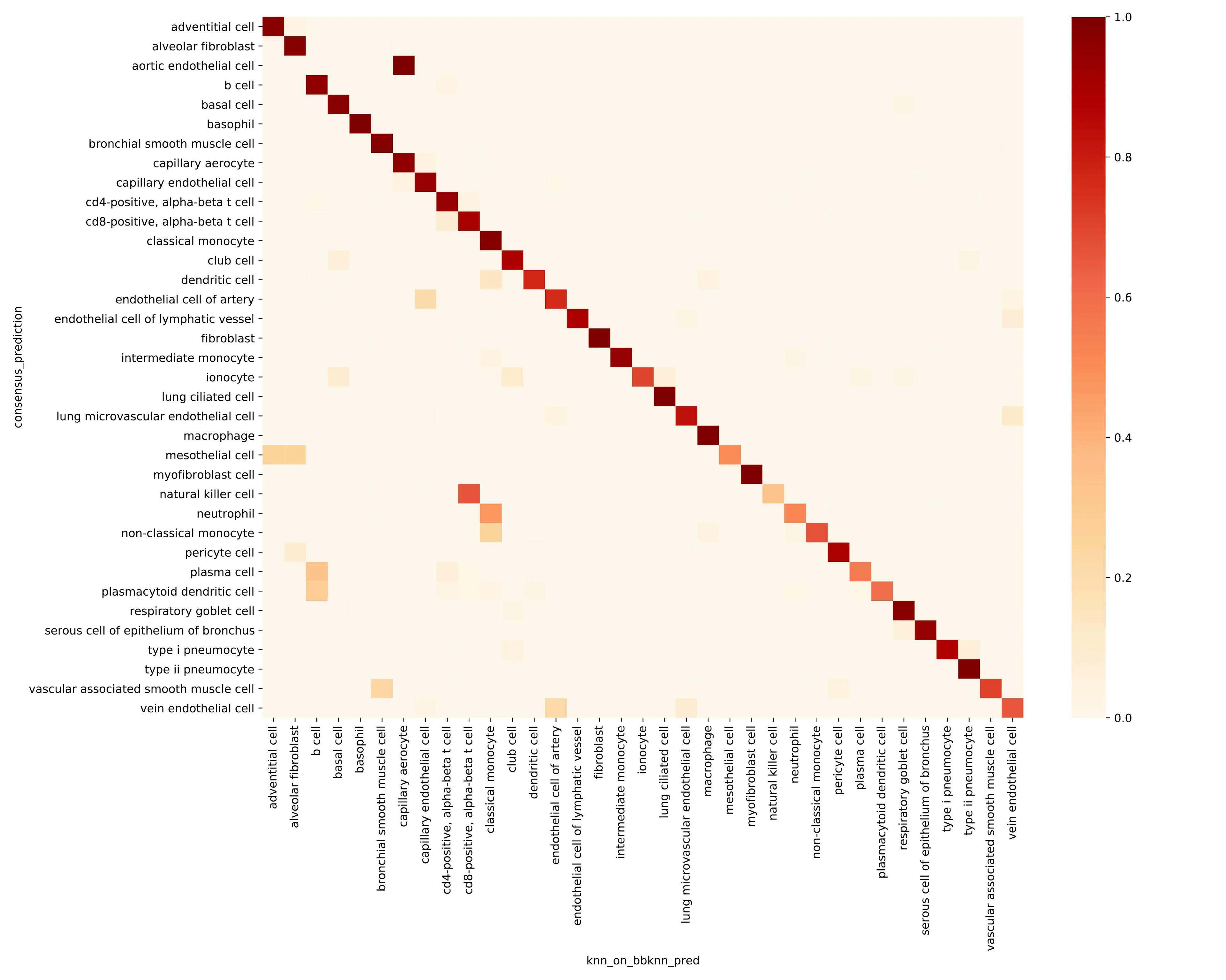
For each method, we compare its prediction to the consensus prediction. Confusing matrix heatmap where rows represent the svm prediction and columns are the majority vote predictions. The off-diagonal elements indicate cell types that are difficult to predict.

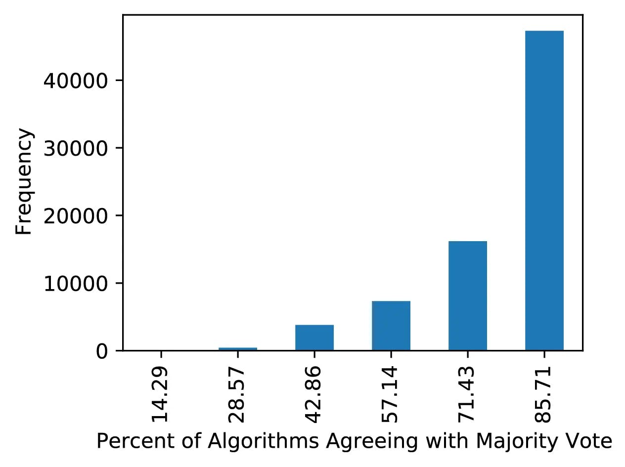
Number of cells that percent algorithms agree on as a histogram.

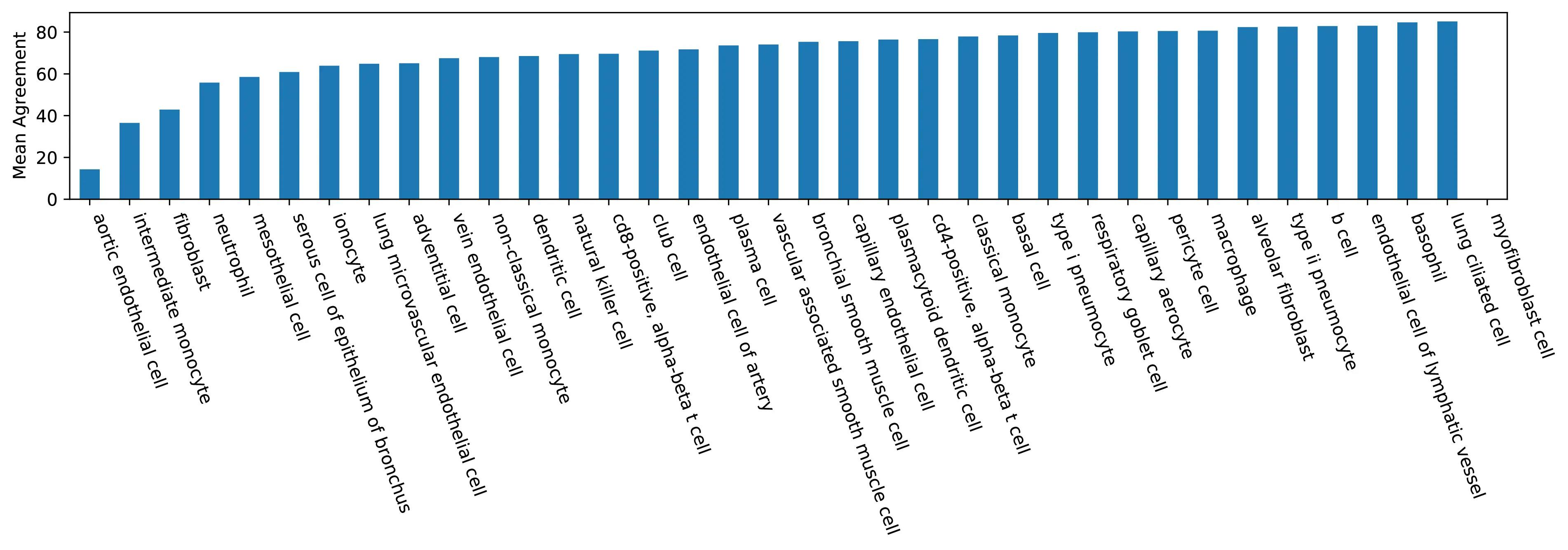
Mean agreement by cell type as a histogram.

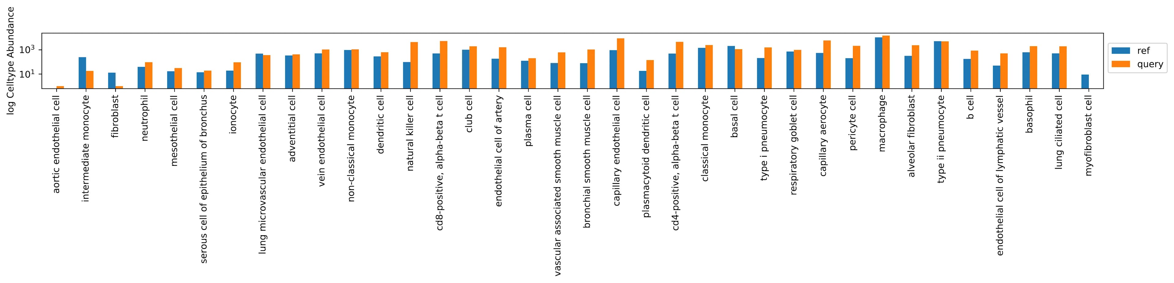
The cell types abundance distribution comparing the reference and query dataset as a paired histogram (color corresponding to dataset).